Visualization

⟵ Previous: Dimensionality Reduction & Clustering Next: Geographic Analysis ⟶

Video Tutorial

The following video tutorial demonstrates some of the ways you can visualize mFISH data.

See code below for some basic plotting functions.

Plotting Functions

Geographic Space

######### STEP 4: PLOTTING #########

### GEOGRAPHIC SPACE with plotSpace()
#plot in space - automatically coloured by cluster
plotSpace(myobj)

#optional args to group by section, or other variable (eg cluster)
plotSpace(myobj, group.by = 'cluster')

#Plot by metadata values
library(dplyr)

Attaching package: 'dplyr'

The following objects are masked from 'package:stats':

    filter, lag

The following objects are masked from 'package:base':

    intersect, setdiff, setequal, union

myobj@metaData <- mutate(myobj@metaData, virus=ifelse(LEC>3, 'LEC', ifelse(RSC>3, 'RSC', 'None')))
plotSpace(myobj, colour.by = "virus")

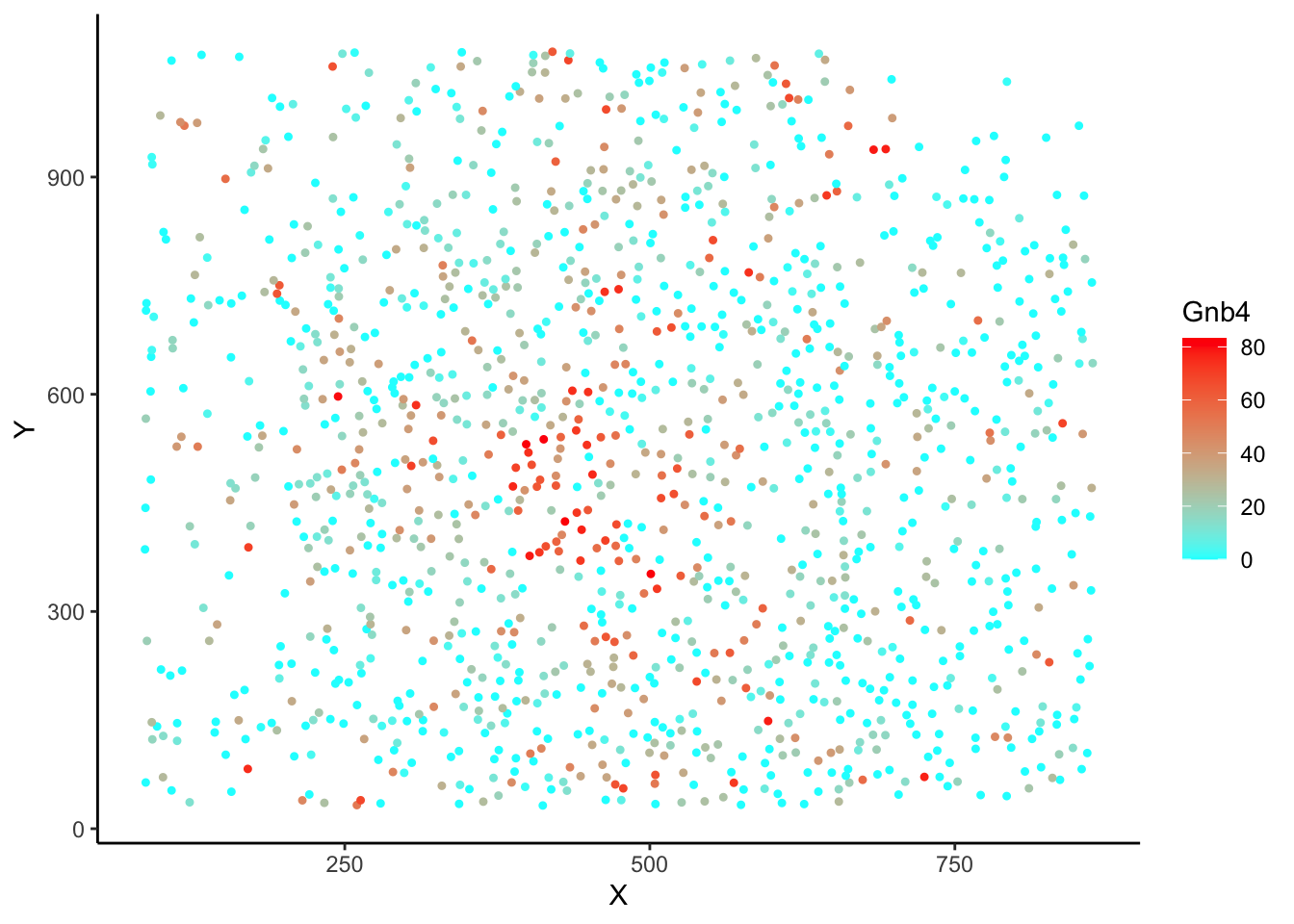
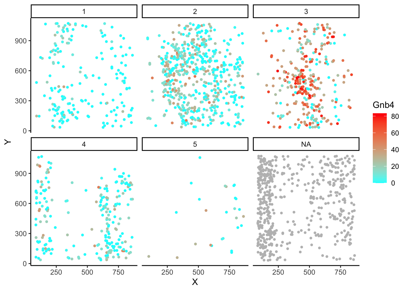
#plot in space but change to a gene or metadata value
plotSpace(myobj, colour.by = 'Gnb4', include.fil = F)

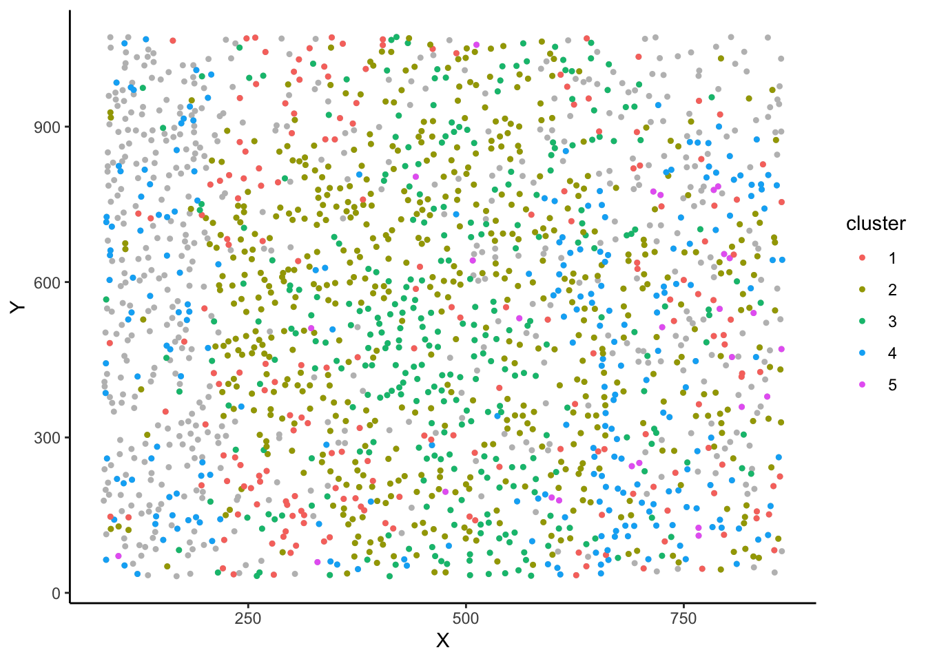
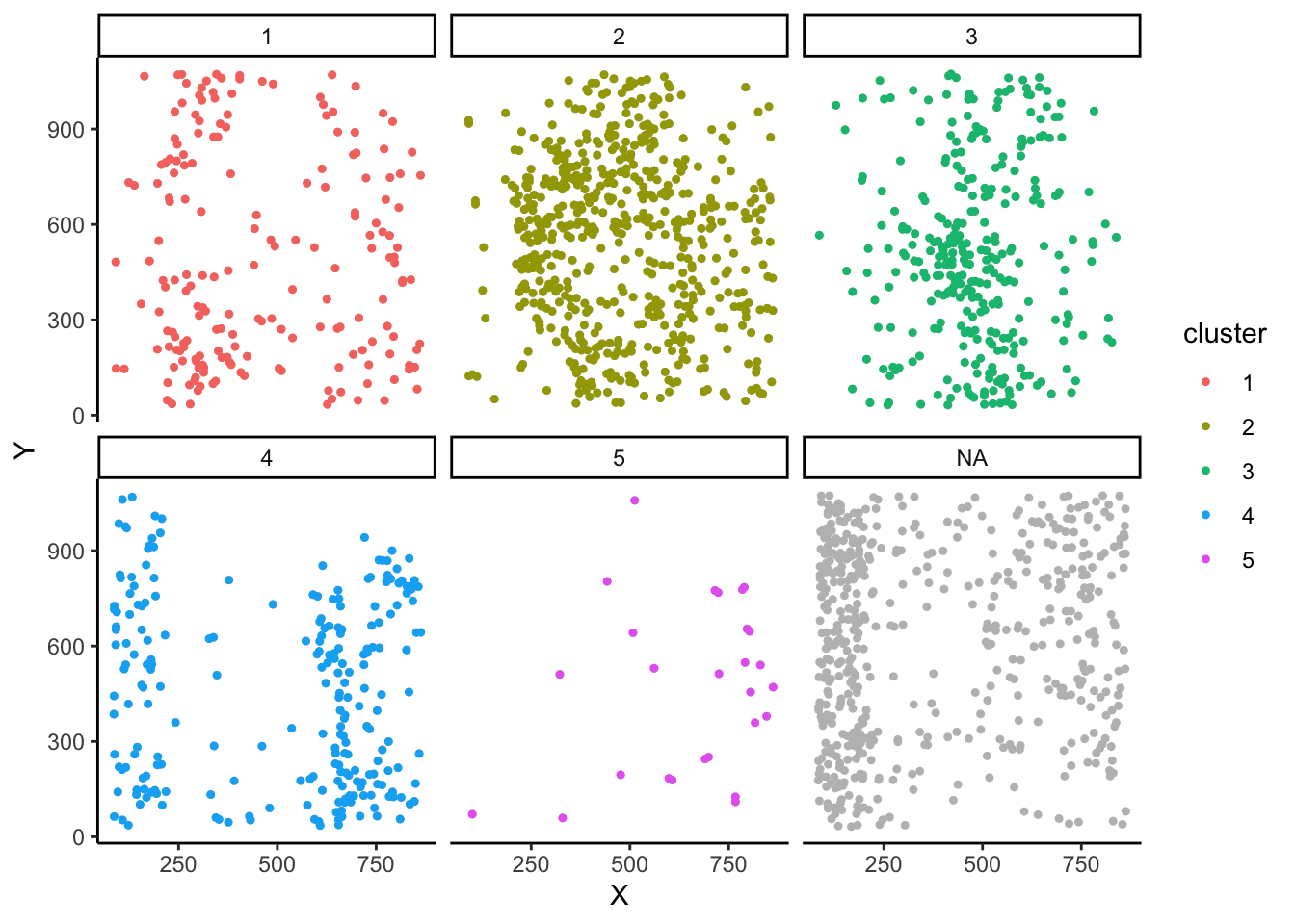
#plot in space with separation by cluster (group.by is useful for viewing multiple sections as well)
plotSpace(myobj, group.by = 'cluster', colour.by = 'Gnb4')

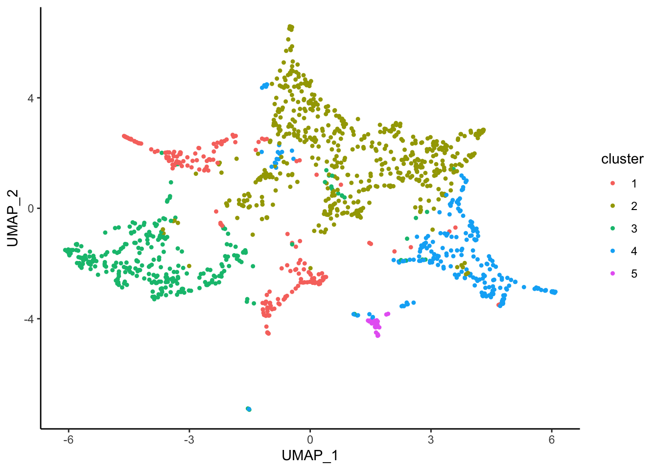
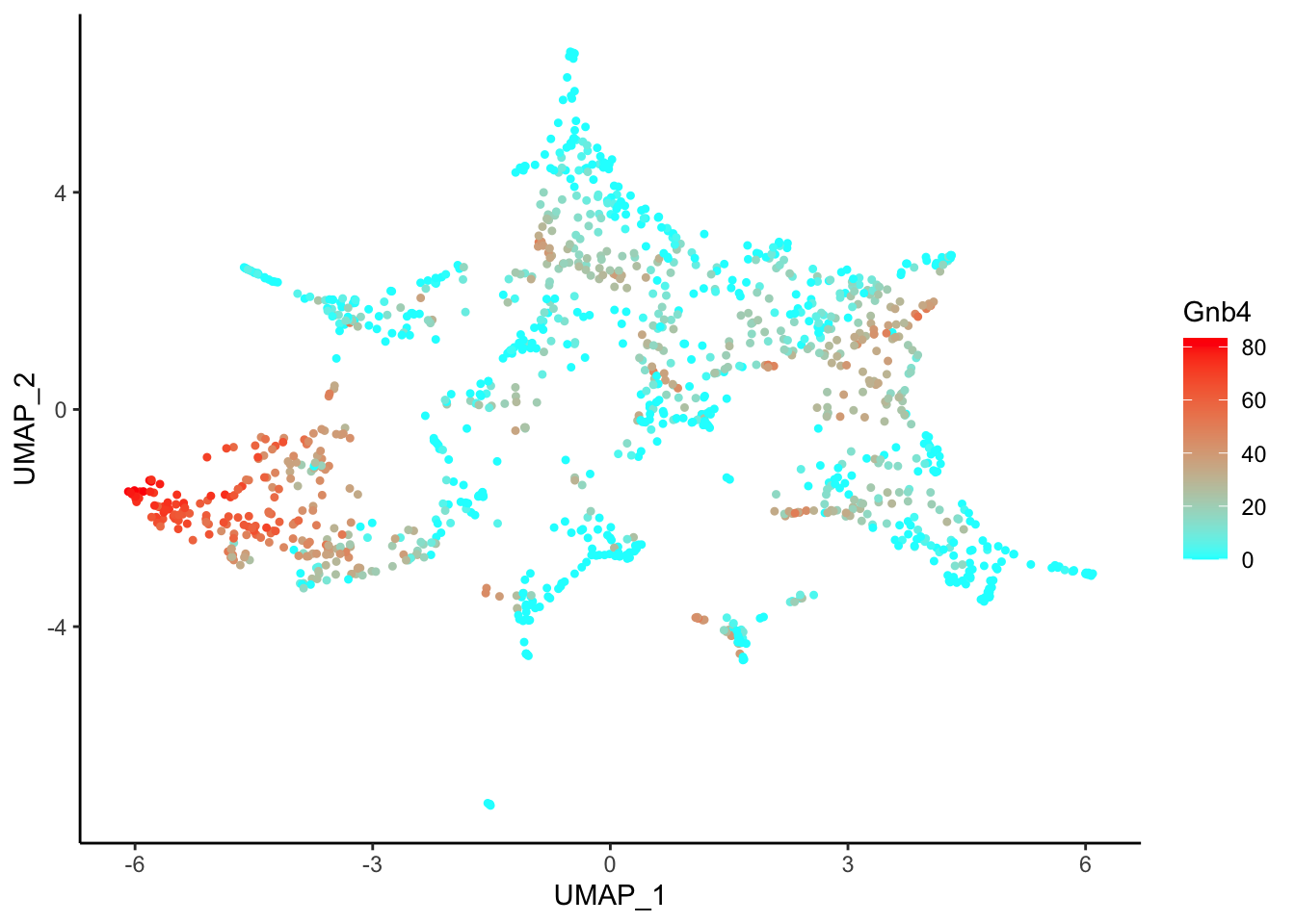
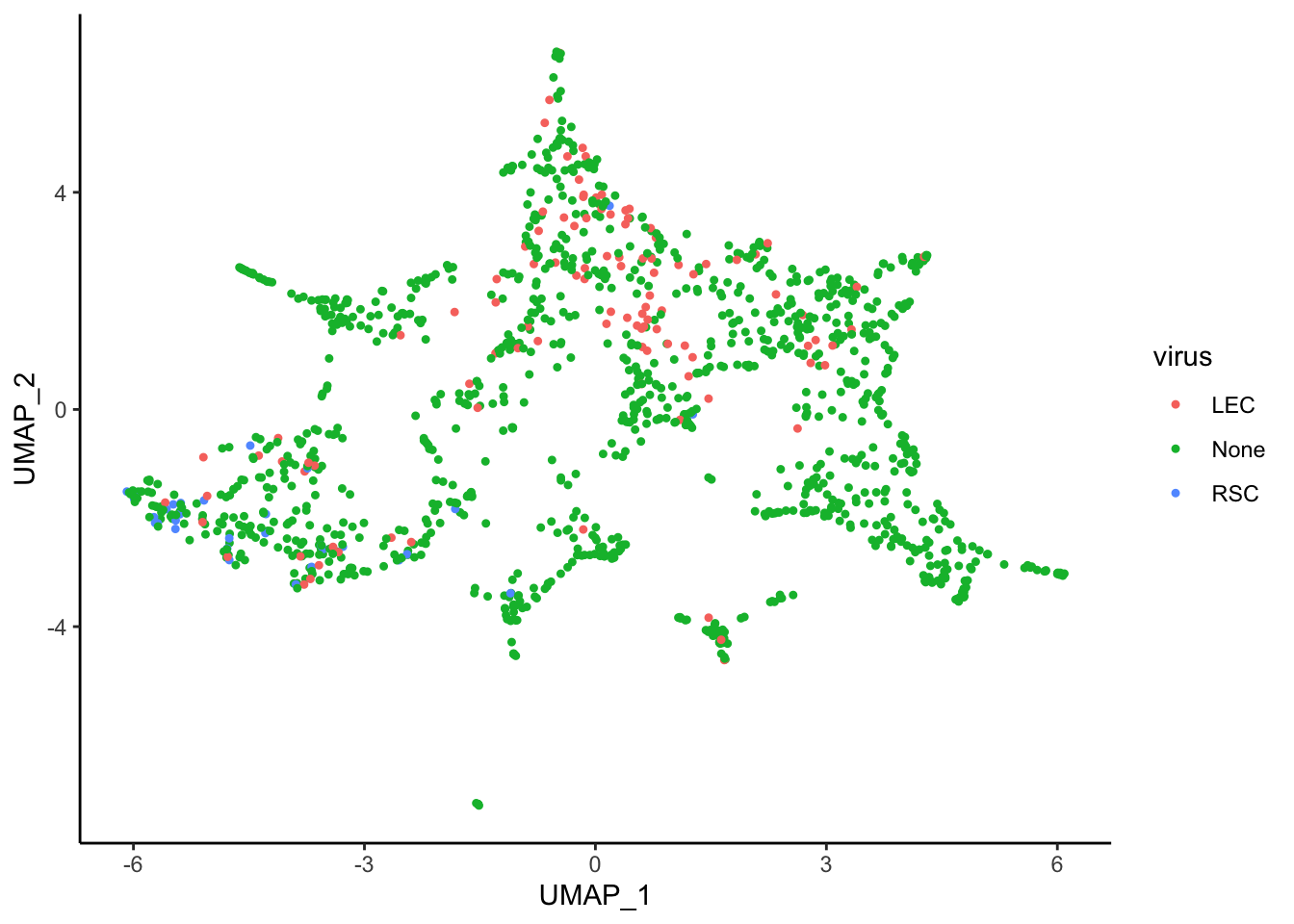
Dimensionally Reduced Space

### DIM REDUCED SPACE with plotDim()
#auto coloured by cluster
plotDim(myobj)

#option to colour by gene/metadata 
plotDim(myobj, colour.by='Gnb4')

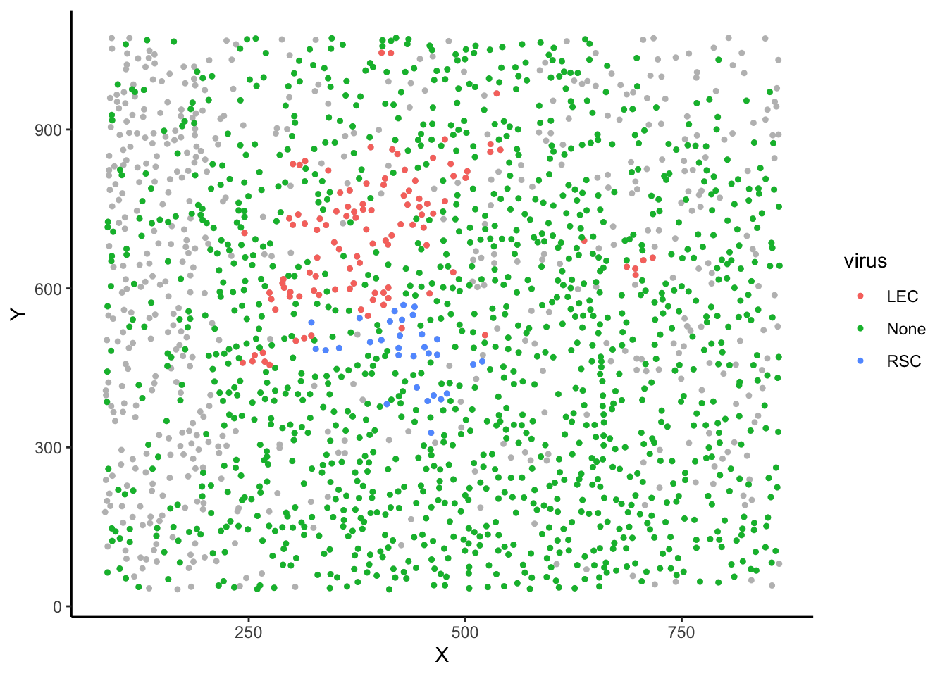
plotDim(myobj, colour.by = 'virus')

Gene Expression Box Plots

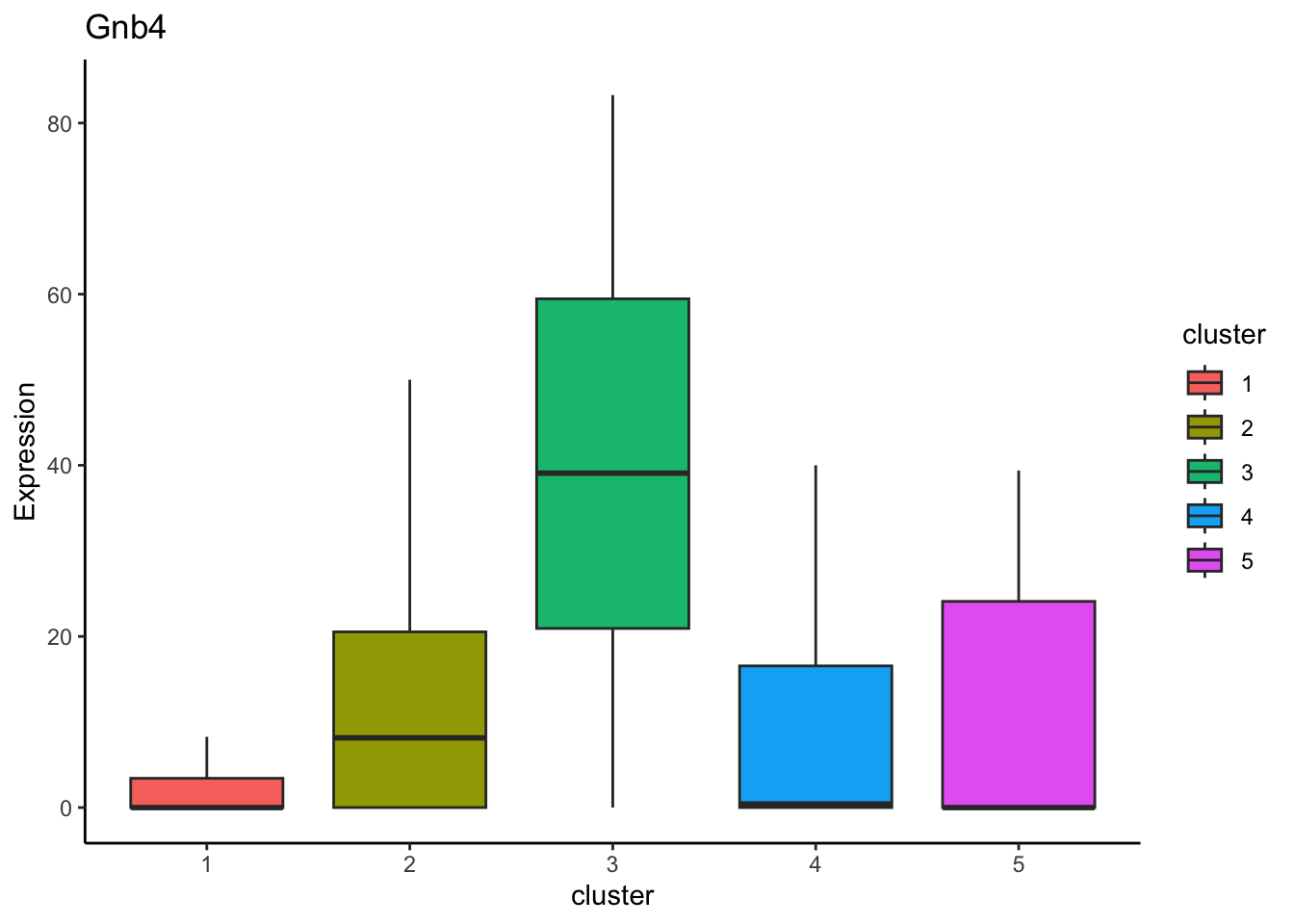
### MARKER GENE BOX PLOTS

#Plot a gene's expression across clusters
geneBoxPlot(myobj, 'Gnb4')

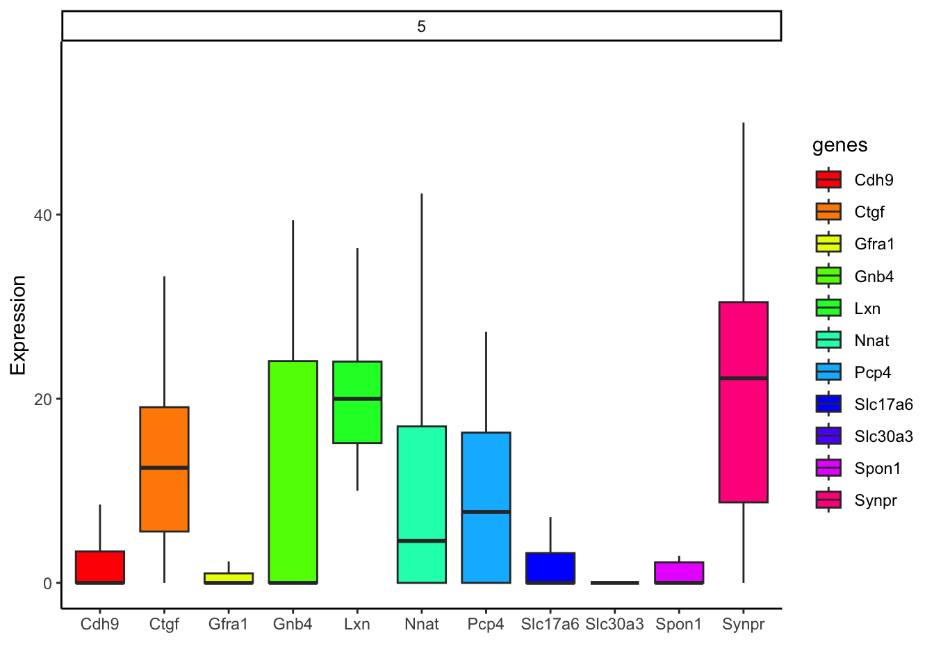
#Plot the gene expression profile of a specified cluster
clusterBoxPlot(myobj, clus='5')

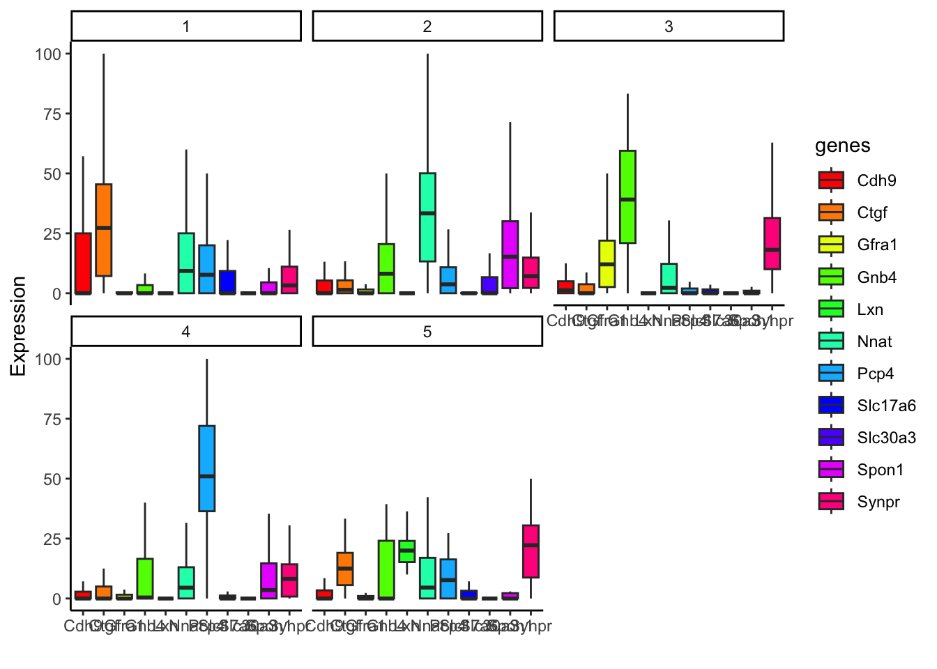
#or simply plot the gene expression for every cluster
clusterBoxPlot(myobj)

⟵ Previous: Dimensionality Reduction & Clustering Next: Geographic Analysis ⟶